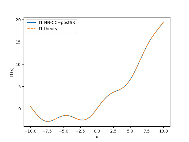
Example 1: Function y=f(x)

This example defines a 1D function f(x) and uses three different methods (polynomials, neural networks, and symbolic regression) to fit the function using the PyCC library.

import pycc
import numpy as np
import pandas as pd
import matplotlib.pyplot as plt
import matplotlib.ticker as ticker

# --- Parameters ---
alpha  = 1.0
beta   = 0.2
delta  = 0.1
# --- Function to discover ---
def F1(x):
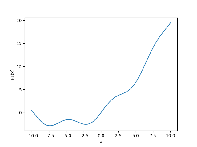
    return alpha*x + delta * x**2 + np.sin(x)
# --- Generating data to train models ---
x_span  = (-10, 10)
x_data  = np.linspace(*x_span, 1000)
F1_th  = F1(x_data)
plt.figure()
plt.plot(x_data,F1_th)
plt.xlabel("x")
plt.ylabel("F1(x)")
plt.show()
# --- Define DataFrame for training models ---
df = pd.DataFrame({
    'x1': x_data,
    'F1_th':F1_th
})
print(df.head())

################################ training model stage #############################
# Define the hypotesized equations to discover
equations=['F1_th = f1(x1)']

########################################
          #### method Poly  ####
########################################
print("computing Poly")
params_poly={
  'scaling': True,
  'constraints': [
        #{'constraint': 'f1(0)=0'},#,'penalty':1e2},
        #{'constraint': 'f2(0)=0'},
        #{'constraint': 'f1 odd'},
        #{'constraint': 'f2 odd'}
    ],
  #'eq_weights':[1.0,0.0]
}
models, evals , scalar_coefs = pycc.train(
    df=df,
    equations=equations,
    method='Poly', #method='Poly_linear',
    params=params_poly
)
x_f1_cc, f1_cc = evals
plt.figure()
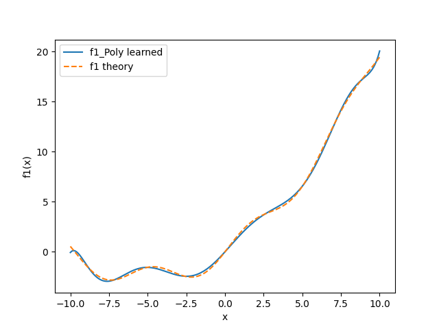
plt.plot(x_f1_cc, f1_cc, label='f1_Poly learned')
plt.plot(x_data,F1_th, '--', label="f1 theory")
plt.xlabel('x')
plt.ylabel('f1(x)')
plt.legend()
plt.show()


########################################
          #### method SymbR  ####
########################################
params_SymbR = {
  'pysr': {
    'niterations': 100,
    'unary_operators': ['tanh','sin','cos'],
    'binary_operators': ['+','-','*'],
    'maxsize': 12,
    'populations':20,
    'model_selection': 'accuracy', # 'best' , 'accuracy' , 'score'
    'verbosity': 0
  },
  'N_fit_points': 200,
  'max_iterations': 15,
}

models, evals , scalar_coefs = pycc.train(
    df=df,
    equations=equations,
    method='SymbR',
    params=params_SymbR
)


print("\nFinal symbolic regression results:")
for fname, out in models.items():
    best_model = out['pysr_model'].get_best()['equation']
    print(f"{fname}(x0) ≈ {best_model}")
    print(f"{fname}(x0) ≈ {out['pysr_model']}")
    print(f"{fname}(x0) ≈ {out['pysr_model'].sympy()}")


x_f1_cc, f1_cc = evals
plt.figure()
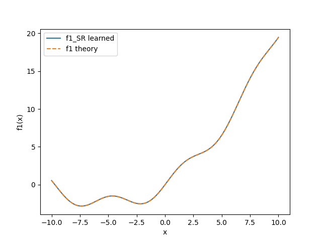
plt.plot(x_f1_cc, f1_cc, label='f1_SR learned')
plt.plot(x_data,F1_th, '--', label="f1 theory")
plt.xlabel('x')
plt.ylabel('f1(x)')
plt.legend()
plt.show()

########################################
          #### method NN  ####
########################################
constraints = [
    {'constraint': 'f1(0)=0', 'penalty': 1e-2},
   #{'constraint': 'f2(0)=0', 'penalty': 1e-2},
    {'constraint': 'f1 odd', 'penalty': 1e-1, 'eval': 'array','Nval_array':100}, # penaly is optional
    {'constraint': 'f2 odd', 'penalty': 1e-1, 'eval': 'array','Nval_array':100}, # eval=data/array array is default
]
parameters_NN = {
    'neurons': 100,
    'lr': 1e-4,
    'epochs': 10000,
    'error_threshold': 1e-6,
    'extrapolation': None,
    'weight_loss_param': 1e1,
}
models, evals, obtained_coefs = pycc.train(
    df,
    equations,
    method='NN',
    params=parameters_NN,
)

x_f1_cc, f1_cc = evals
plt.figure()
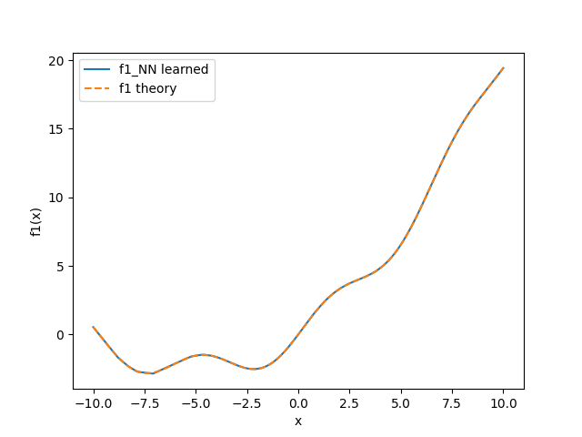
plt.plot(x_f1_cc, f1_cc, label='f1_NN learned')
plt.plot(x_data,F1_th, '--', label="f1 theory")
plt.xlabel('x')
plt.ylabel('f1(x)')
plt.legend()
plt.show()
# Print learned parameters (if any)
if obtained_coefs:
    print("\nLearned scalar parameters:")
    for name, val in obtained_coefs.items():
        print(f"{name} = {val.item():.4f}")



# Obtain an analytical expression for the identified function
pysr_settings = {
    'niterations': 100,
    'populations': 20,
    'binary_operators': ['+', '*', '-'],
    'unary_operators': ['tanh', 'sin','cos'],
    'maxsize': 20
}
# Define the 'params' dictionary for the post-processing function
post_process_params = {
    'evals': evals,
    'pysr': pysr_settings,
    'plot': True,  # This will show the plots of the fits
    'n_eval': 200,
}
# Run the post-processing
models_sr,evals_sr = pycc.post_processing(equations, method='SymbR', params=post_process_params)

print("\nFinal symbolic regression results:")
for fname, out in models_sr.items():
    best_model = out['pysr_model'].get_best()['equation']
    print(f"{fname}(x0) ≈ {best_model}")
    print(f"{fname}(x0) ≈ {out['pysr_model']}")
    print(f"{fname}(x0) ≈ {out['pysr_model'].sympy()}")


x_f1_cc, f1_cc = evals_sr
plt.figure()
plt.plot(x_f1_cc, f1_cc, label='f1 NN-CC+postSR')
plt.plot(x_data,F1_th, '--', label="f1 theory")
plt.xlabel('x')
plt.ylabel('f1(x)')
plt.legend()
plt.show()