Usage

First time? We recommend starting with our Google Colab Notebook! https://colab.research.google.com/drive/136FvEwMsxLayhimgtI4Jx_IWR8l-dy-s

The following example shows:

1. How to simulate a stick-slip second order system using pycc.simulate() and generate the input database.

2. How to identify the model (train) using the NN-CC method pycc.train()

3. How to simulate the identified model pycc.simulate()

import pycc
import numpy as np
import pandas as pd
import matplotlib.pyplot as plt

# 1a) define parameters and functions
alpha=1.0;beta=0.2;delta=0.1;Omega=1.0;
x0=0.0;v0=0.0; y0=[x0,v0] # initial conditions
t_span=(0, 20); t_eval=np.linspace(*t_span, 1000)
def F1_th(x_dot):
    return delta * x_dot + 0.5 * np.tanh(500*x_dot)
def F2_th(x):
    return alpha * x + beta * x**3
def F_ext(t):
    return np.cos(Omega * t)

# 1b) define equation
eqs_th = ['x1_dot = x2',
          'x2_dot = F_ext - f1(x2) - f2(x1)']

# 1c) define simulation parameters
params_th = {
    't_span': t_span,
    'y0': y0,
    't_eval': t_eval,
    'method': 'LSODA',
    'local_funcs': {'f1': lambda t: F1_th(t),'f2': lambda t: F2_th(t),'F_ext': lambda t: F_ext(t)}
}
# 1d) integrate forward the theoretical equation
sol,derivatives = pycc.simulate(eqs_th,method="Theoretical", params=params_th)

# 1e) extract data from theoretical solution
time_data    = sol.t
x1_data      = sol.y[0]
x2_data      = sol.y[1]
x1_dot_data  = derivatives[0]
x2_dot_data  = derivatives[1]
F_ext_val    = F_ext(time_data)

# define database for training
df = pd.DataFrame({
    'x1':x1_data,
    'x2':x2_data,
    'x1_dot':x1_dot_data,
    'x2_dot':x2_dot_data,
    'F_ext': F_ext_val
})

# 2a) propose equations to use for identification (fi functions and ai parameters).
eqs = [
     'x1_dot = x2',
     'x2_dot = F_ext - f1(x2) - f2(x1)'
]
# 2b) define constraints (optional)
constraints = [ # adding prior known information
    {'constraint': 'f2(0)=0'},
    {'constraint': 'f1 odd'},
    {'constraint': 'f2 odd'},
]
# 2c) define training parameters (optional)
params_NN = {
    'neurons': 100,
    'layers':3,
    'lr': 1e-4,
    'epochs': 2000,
    'error_threshold': 1e-6,
    'extrapolation': None,
    'device':'cpu',
    'weight_loss_param': 1e-3,
    'constraints': constraints,
}
# 2d) train/fit/identify the model
models, evals, obtained_coefs = pycc.train(df, eqs,method='NN', params=params_NN)

# plotting obtained functions f1 and f2
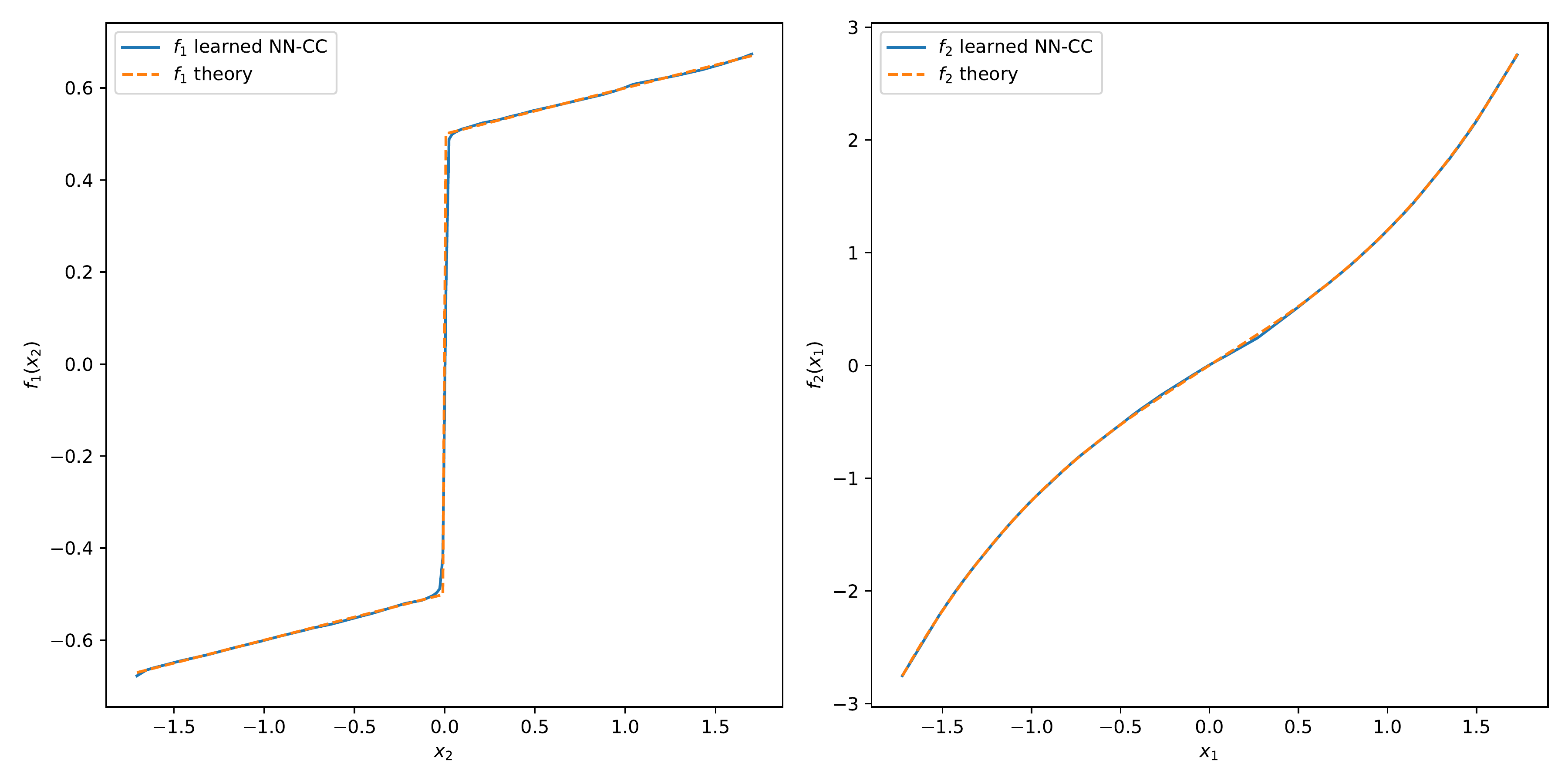
x_f1_cc, f1_cc, x_f2_cc, f2_cc = evals
fig, ax = plt.subplots(1, 2, figsize=(12, 6))
ax[0].plot(x_f1_cc, f1_cc, label='$f_1$ learned NN-CC')
ax[0].plot(x_f1_cc, F1_th(x_f1_cc), '--', label="$f_1$ theory")
ax[0].set_xlabel('$x_2$')
ax[0].set_ylabel('$f_1(x_2)$')
ax[0].legend()
ax[1].plot(x_f2_cc, f2_cc, label='$f_2$ learned NN-CC')
ax[1].plot(x_f2_cc, F2_th(x_f2_cc), '--', label="$f_2$ theory")
ax[1].set_xlabel('$x_1$')
ax[1].set_ylabel('$f_2(x_1)$')
ax[1].legend()
plt.tight_layout()
plt.show()

# Print learned parameters (if any)
if obtained_coefs:
    print("\nLearned scalar parameters:")
    for name, val in obtained_coefs.items():
        print(f"{name} = {val.item():.4f}")

### Simulation using the NN models

print("simulation with NN simul")
# 3a) define simulation parameters
params_NN_simul = {
    'models': models,
    'obtained_coefs': obtained_coefs,
    'local_funcs': {'F_ext': lambda t: F_ext(t)},
    't_span':t_span,
    'y0': y0,
    't_eval': t_eval,
    'method': 'LSODA',  # solve_ivp
    'atol': 1e-8,
    'rtol': 1e-6,
    'check_nan': True
}
# 3b) integrate identified equations
sol,_ = pycc.simulate(eqs, method='NN', params=params_NN_simul)
print("Integration success:", sol.success)

time_sim=sol.t
x1_sim=sol.y[0]
x2_sim=sol.y[1]

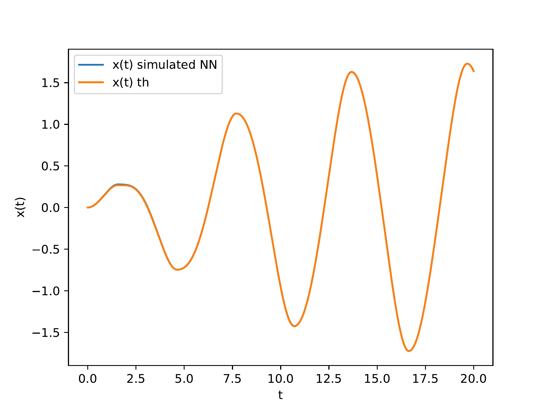
# Identified vs theoretical solution
plt.figure()
plt.plot(time_sim, x1_sim, label="x(t) simulated NN")
plt.plot(time_data, x1_data, label="x(t) th")
plt.xlabel('t')
plt.ylabel('x(t)')
plt.legend()
plt.show()