👋 PyCC
PyCC.id: A package for hypothesis-driven equation discovery with structural identifiability
PyCC.id (or simply PyCC) is a Python library designed for equation discovery, specifically aiming to obtain ordinary differential equations (ODEs) from time-dependent data. The library is built on a hypothesis-driven methodology, enabling users (such as researchers and engineers) to easily incorporate prior domain knowledge into the discovery process. This hypothesis-driven approach empowers users to explicitly propose a specific skeleton (or a structural family of models) based on their expertise, and rigorously test whether that proposal is consistent (or not) with the given data.
By centering the workflow around hypothesis testing, PyCC provides a structured framework to help tackle several common challenges in equation discovery, such as identifiability, interpretability, and physical consistency. It also enables a modular approach that allows the use of complex functional representations by taking advantage of universality theorems from neural networks while maintaining transparency. These topics are briefly discussed below:
🎯 Why PyCC
i) Identifiability
When inferring dynamical equations from experimental data (which is often noisy and sampled) multiple distinct mathematical models routinely fit the observations with comparable accuracy. This leads to ambiguities in model selection, a core issue known as the identifiability challenge. This ambiguity is intrinsically connected to the ill-posed nature of the inverse problem. Attempting to reconstruct the true physical laws from a specific data realization (constrained by sampling rate, observation window, and specific initial conditions) often results in practically unidentifiable underlying equations using generic, structure-agnostic methods.
PyCC circumvents this identifiability challenge by empowering the user to guide the search with prior physical knowledge or specific hypotheses. Specifically, the library allows the user to force a structural ‘skeleton’ and to easily impose additional properties or constraints to ensure the discovered models are physically sound.
The choice of the structural skeleton directly affects identifiability: while certain skeletons possess structural identifiability, others can result in non-identifiable or ambiguous representations. When the skeleton is shown to be theoretically identifiable in phase space (see, e.g., [Gon26b]), PyCC offers a formal framework to analyze if the proposed equation is consistent with the data or should be discarded and reformulated. Consequently, it enables the validation or elimination of hypothesized models, providing a clear pathway through the challenge of identifiability.
ii) Interpretability and physical consistency
Beyond identifiability, a major challenge in data-driven modeling is the interpretability of the obtained models. Even if a complex mathematical formulation fits the data perfectly, its structure can be too opaque to extract meaningful physical insights. This lack of interpretability obscures the underlying physics, leaving practitioners (at best) with accurate predictions but no understanding of the system structure.
To explicitly address this issue, PyCC relies on the concept of characteristic curves (CCs). This concept is grounded in the concept of the constitutive relation of an element. The constitutive relation links two variables and (in the scalar case) can be parametrized by a one dimensional (1D) curve known as the CC of the corresponding element. Thus, the CC completely defines the element. PyCC offers a flexible and easy notation to help the user to define the equation skeletons that incorporate unknown 1D functions and/or parameters to be discovered. If the user defines skeletons where the unknown functions correspond to the CCs of the system, the functions themselves have a physical meaning.
To illustrate this, we consider three skeleton structures in the following (which are also structurally identifiable, as shown in [Gon23]:
First-order systems:
Here, \(f_1\) and \(f_2\) may correspond to a nonlinear resistor and inductor, respectively, but could also be related to viscoelastic materials and nonlinear mechanical damping (see, e.g., [Gon23] and [Gon24]).
Second-order systems with position-dependent friction:
In this structure, \(f_1\) represents a position-dependent friction element, and \(f_2\) is an elastic component (see, e.g., [GL25] and [Gon26b]).
Second-order systems with velocity-dependent friction:
Here, \(f_1\) and \(f_2\) capture velocity-dependent friction and elastic elements, respectively (see, e.g., [GL25] and [Gon26b]).
Additionally, the PyCC approach allows the users to visualize the CCs to verify their hypotheses or define new ones. This transforms an abstract mathematical representation into a direct visual tool, significantly enhancing interpretability.
For instance, consider the second-order systems with velocity-dependent friction defined above. Suppose that after using some training method, the obtained CC results in visually a straight line, thus, it is an indication that the elastic element is linear (in this case, we could add this as an additional hypothesis and retrain the model). If, instead, the CC results in a parabola, it is an indication that the elastic element is nonlinear (based on the obtained CC, we can add new hypotheses and retrain the model). This matching between the functions of the models and individual elements of the system ensures the final model maintains physical consistency and allows the user to incorporate prior insights easily.
This transparent approach based on CCs has a simple but profound implication: the objective shifts from finding precise parameter values for the CCs expanded in some basis functions to finding the functional form of the CCs themselves.
As a consequence, it allows us to use fitting methods with thousands of parameters such as neural networks (NNs) but maintaining physical consistency and interpretability.
Summary:
Traditional approach: “Find the coefficients \(k\) and \(c\) assuming linear dynamics.”
PyCC approach: “Find the shapes of the stiffness and damping curves.”
iii) Modularity, Universality and Transparency
Because PyCC prioritizes discovering the shape of these CCs rather than fitting predefined coefficients, the specific parametric form of the curves (e.g., whether they are polynomial, exponential, or trigonometric) does not need to be postulated a priori. This flexibility unlocks a highly modular framework that is ideal to compare different paradigms in data-driven modeling.
For instance, the CCs can be parameterized using universal approximators, such as Neural Networks (NNs). This specific implementation (referred to as the NN method) is particularly powerful for discovering complex physical laws. Backed by universal approximation theorems, the model can adapt to any continuous shape and also capture intricate dynamics such as sharp transitions and non-smooth behaviors without requiring prior mathematical intuition about the functional form.
Crucially, this approach preserves transparency. While NNs can be considered as opaque “black boxes” in high-dimensional settings, PyCC restricts them to learning strictly 1D functions. A “black box” with a single input and a single output is effectively a curve that can be plotted, visually inspected, and physically understood.
Note
The Core Philosophy: Instead of asking “What is the global equation?”, PyCC asks “Given this physical structure (skeleton), what are the specific shapes of the CCs?” These curves are the constitutive relations of the system; once they are identified, the identification problem is effectively solved.
💡 The PyCC approach: A schematic workflow
PyCC frames discovery as a hypothesis-testing loop. The practitioner proposes a structure (e.g., “Is this a friction-based oscillator?”), and the library determines the optimal shapes of the internal functions in order to decide if the hypothesized structure is coherent with the data or should be modified.
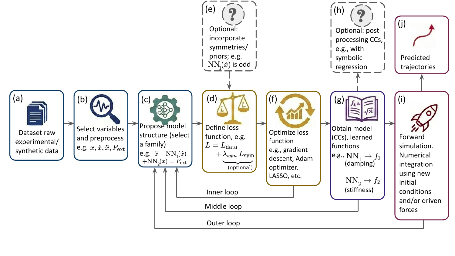
Figure 1: The PyCC workflow. (a-c) A hypothesized model structure is proposed. (d-f) A representation for the CCs is selected (via NN, SymbReg, etc.), and optional constraints are defined to be minimized jointly with the data loss term. (g-j) The resulting curves are inspected for physical validity and forward simulations are performed with the obtained models. Adapted from arXiv:2601.21720 [Gon26]
The workflow proceeds in three main stages:
- 1. Hypothesis & Setup (a-c)
The process begins with raw experimental or synthetic data (a). The practitioner selects the relevant state variables (e.g., position \(x\), velocity \(\dot{x}\), and external force \(F_{ext}\)) (b). Crucially, instead of assuming a “black box,” a Structural Skeleton is proposed (c). For example, one might hypothesize a second-order oscillator structure: \(\ddot{x} + f_1(\dot{x}) + f_2(x) = F_{ext}(t)\).
- 2. Physics-Informed Optimization (d-f)
The library constructs a loss function (d) to fit the data. An important feature of PyCC is the ability to inject prior physical knowledge or hypotheses (e) directly into this stage.
Example: If you hypothesize that the friction curve should be symmetric, you can enforce this constraint—for example, by stating that \(f_1(\dot{x})\) must be an odd function.
The optimizer (f) (e.g., Adam/AdamW for Neural Networks) finds the functions that best satisfy both the data and these physical constraints.
Inner Loop: If the obtained loss function after optimization is not sufficiently small, it suggests the hypothesized structural skeleton cannot capture the physics. The workflow returns to (c) to propose a different model family.
- 3. Discovery & Validation (g-j)
The output is not just a prediction, but the CCs themselves (g).
Interpretability & The Middle Loop: You can plot the CCs to visually inspect the physics. For instance, for the second-order example mentioned above, \(f_1\) represents a damping force and \(f_2\) a stiffness force.
Consistency Check: If the learned CCs look unphysical or vary significantly across different datasets (lack of invariance), the hypothesis is rejected. This triggers the Middle Loop, returning to model selection (c).
Post-Processing (h): Optionally, these CCs can be fed into a Symbolic Regression tool to recover analytical equations (e.g., finding that \(f_2(x) \approx kx + \beta x^3\)). PyCC provides a built-in interface that calls PySR code to perform this translation automatically.
Validation (i-j): Validation extends beyond verifying the shape of the CCs; the final rigorous test is provided by forward simulations. The model is tested against new initial conditions or external forces to ensure it generalizes to unseen data or unexplored regions of the phase space. If these simulations fail to adequately reproduce the system dynamics, the process returns to the model selection stage (c) (via the Outer Loop) to revise the structural hypothesis and/or constraints.
🔬 Application example to a second order system
To illustrate the application of the workflow, consider the task of identifying a second-order system with a velocity-dependent friction force and external driving force. The practitioner starts by hypothesizing a second-order structural skeleton:
This equation implies that the system is governed by two CCs: i) A damping force \(f_1\) that depends solely on velocity. ii) A restoring force \(f_2\) that depends solely on position.
Figure 2 illustrates how this hypothesis is translated into the PyCC internal architecture. In this example, we parameterize the CCs as Neural Networks (thus the method is referred to as NN-CC), but other parameterizations are available.
The package handles the structural implementation automatically, allowing the practitioner to focus solely on defining the hypothesized equation (see Usage tab).
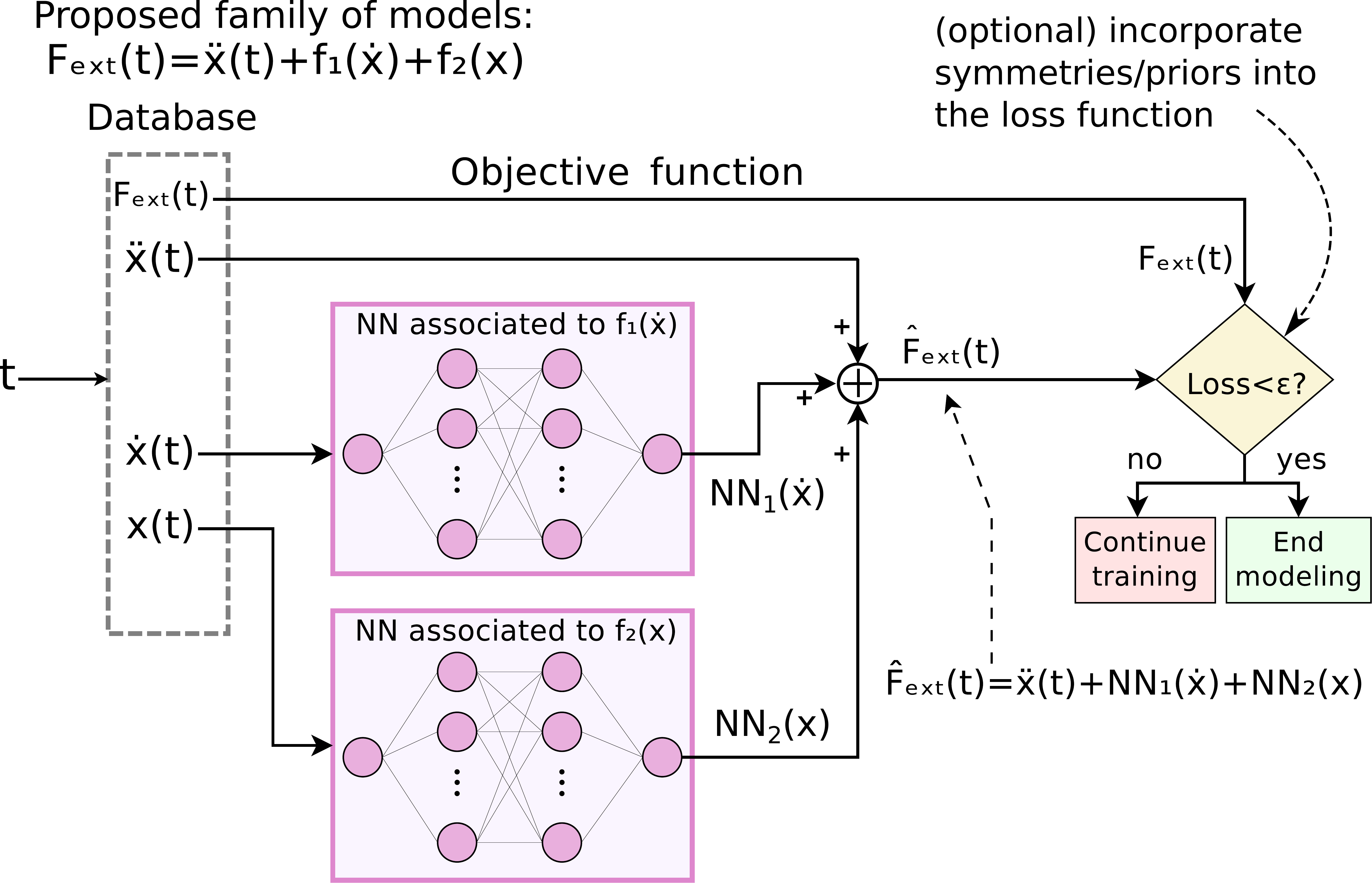
Figure 2: The architecture for a second-order system. Two independent neural networks (\(\text{NN}_1\) and\(\text{NN}_2\) ) approximate the unknown CCs.\(\,\text{NN}_1\) sees only velocity, and\(\,\text{NN}_2\) sees only position. Their outputs are summed to match the hypothesized structure.
The internal architecture can be basically characterized by:
A dedicated estimator ( \(\text{NN}_1\) ) receives only the velocity \(\dot{x}\) to learn the shape of \(f_1\).
A dedicated estimator ( \(\text{NN}_2\) ) receives only the position \(x\) to learn the shape of \(f_2\).
Why this architecture matters:
Crucially, this architecture enforces the properties of uniqueness, interpretability, and physical consistency mentioned above. This guarantees that, upon convergence, the solution is unique: \(\text{NN}_1\) effectively converges to \(f_1\) and \(\text{NN}_2\) to \(f_2\), avoiding any ambiguity in the identification of the functions, as discussed in arXiv:2601.21720.
📝 Formalism
Equation discovery (which can be considered as a subfield of system identification) is the process of finding the underlying governing equations of a system from observational data. A wide variety of systems (ranging form physical and engeneering to biological, chemical, economic and social), the dynamics can be described by a set of first-order ordinary differential equations (ODEs):
where \(\mathbf{x}=\mathbf{x}(t)\) is the state vector containing the dynamical variables (e.g., position, velocity). The explicit time-dependence can always be considered as external driving forces \(\mathbf{F}_{ext}(t)\) , giving the equation:
Identifying the global function \(\mathbf{F}\) directly often results in “black-box” models that often lack physical insight and lead to ambiguities under noise or other experimental conditions. PyCC.id avoids this by decomposing \(\mathbf{F}\) into interpretable building blocks, mimicking the way a scientist builds a model by isolating phenomena like stiffness or damping beforehand.
Mathematically, we express this decomposition as:
where:
\(\mathbf{G}\) represents a user-defined model structure or template that dictates how the building blocks (the functions \(\{\mathbf{f}\}\) and parameters \(\mathbf{a}\)) are combined to satisfy the proposed equation.
\(\mathbf{x}\) and \(\mathbf{F}_{ext}(t)\) are the inputs for the modeling step. These are the quantities that define the database used for training the models. \(\mathbf{x}\) is the dynamical variable or state of the system; and \(\mathbf{F}_{ext}(t)\) is a set of time-dependent external forces.
;: The parameters to the right of the semicolon (;) are the unknowns to find.\(\{\mathbf{f}\}\) is a set of unknown functions to be discovered (CCs). Each function depends on only a single state variable \(x_i\).
\(\mathbf{a}\): A set of unknown scalar parameters to be discovered, such as mass or other physical coefficients.
The goal of PyCC is to discover the optimal functions \(\{\mathbf{f}\}\) and parameters \(\mathbf{a}\) that best fit the observed data based on a predefined model structure \(\mathbf{G}\).
✨ Key Features
Interpretable Models: Decomposes complex dynamics into simpler, physically meaningful functions.
Flexible Function Parametrization: Supports various techniques to model the CCs, including:
Neural networks (NN-CC) : Utilizes NNs to parameterize the CCs; compatible with multicore CPUs and GPUs from both NVIDIA (CUDA) and Intel (XPU) architectures via PyTorch.
Polynomials (Poly-CC) : Utilizes polynomial basis functions to parameterize the CCs.
Symbolic regression (SymbR-CC) : Utilizes symbolic regression to parameterize the CCs; parallelized for multicore CPU execution using the internal parallelization features of the PySR package.
Physics-informed discovery: Incorporate known physical constraints, such as symmetries (e.g., even and odd functions) or additional conservation laws, to guide the discovery process and ensure robust, physically consistent models.
Interface with standard simulators: Includes an interface with
scipy.integrate.solve_ivp, which is the standard Python tool within the SciPy library used to numerically solve initial value problems (IVPs) for ordinary differential equations (ODEs). This module is fully compatible with all identification methodologies.User-focused design: Offers an API that is both easy to use and highly customizable for advanced research.