Example 5: 2nd-order ODE - Parametric method with post-fine-tuning
The pyCC library also supports an advanced optimization workflow referred to as post-fine-tuning. In this workflow, the code performs a two-step internal procedure. First, it optimizes the predefined model using the entire stream of reference database, exactly as shown earlier in this tutorial. Then, by simply adding extra parameters to the training routine, the code triggers an additional stage where it uses the obtained model to run forward integrations, generating simulated trajectories that are compared to the reference data. Based on this comparison, the code performs a fine-tuning of the model parameters and integrates forward again, thus performing an iterative post-fine-tuning procedure.
import pycc
import numpy as np
import pandas as pd
import matplotlib.pyplot as plt
import matplotlib.ticker as ticker
from scipy.integrate import solve_ivp
from scipy.signal import savgol_filter

# Integration of the theoretical EDO
# We use here the method='Theoretical' using the pyCC library,
# but we could also use standard python integrators,
#
# define parameters
alpha=1.0; beta=0.2; delta=0.1; mu=0.5; omega=1.0; A=1.0
t_span  = (0, 20)
t_eval  = np.linspace(*t_span, 1000)
x0     = 0.0; v0     = 0.0
y0      = [x0, v0]  # initial conditions
# Theoretical functions
def F1(x_dot):
    return delta * x_dot + mu * np.tanh(500*x_dot)
def F2(x):
    return alpha * x + beta * x**3
def F_ext(t):
    return A * np.cos(omega * t)


# In the following:
# 1) we define the equations we want to integrate,
#    (functions must be defined by f_i and params as a_i)
# 2) we define parameters for the integrator,
# 3) we call to pycc to make the theoretical simulation
equations = [
    'x1_dot = x2',
    'x2_dot = F_ext - f1(x2) - f2(x1)'
]
params_th = {
    # we internally use ivp_solve python function with params defined in the following 4 lines
    't_span': t_span,
    'y0': y0,
    't_eval': t_eval,
    'method': 'LSODA',
    # we need to tell to pycc how to find external/local functions
    'local_funcs': {'f1': lambda x: F1(x),'f2': lambda x: F2(x),'F_ext': lambda t: F_ext(t)},
    #'scalar_params': {'a1':2.0}
}
# now use pycc to integrate the EDOs
sol,derivatives = pycc.simulate(equations,method="Theoretical", params=params_th)
# Extract results
time_data   = sol.t # sol is the OdeSolution returned from ivp_solve
x1_data     = sol.y[0] # x1=x(t)
x2_data     = sol.y[1] # x2=x_dot(t)
F_ext_val   = F_ext(time_data)
x1_dot_data = derivatives[0] #x1_dot=x_dot(t)
x2_dot_data = derivatives[1] #x2_dot=x_ddot(t)
F1_th = F1(x2_data)
F2_th = F2(x1_data)

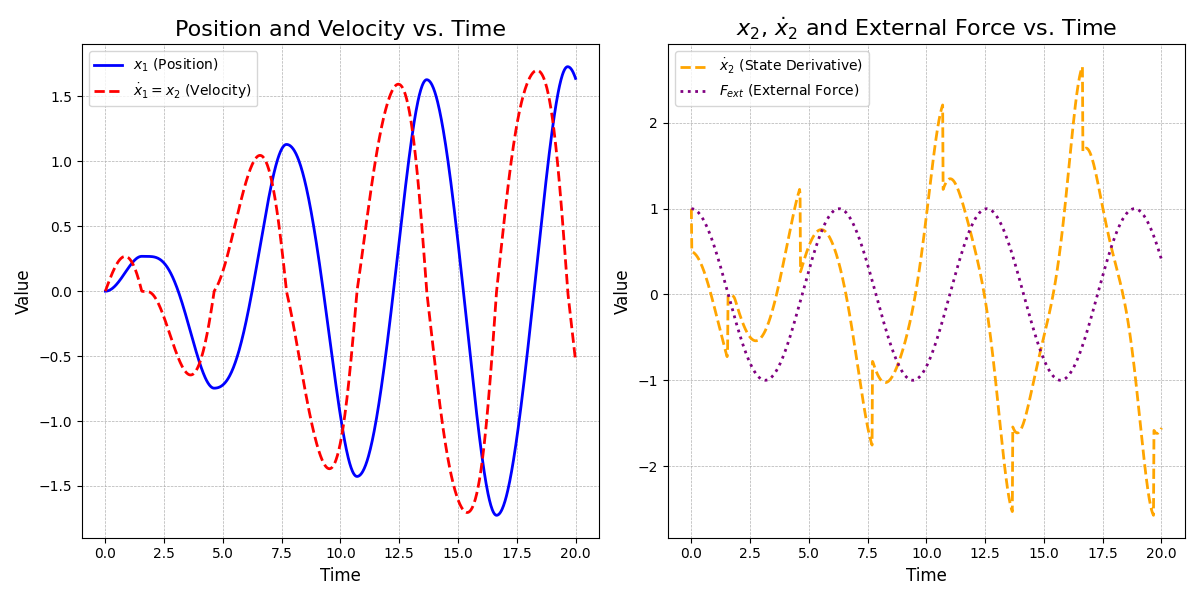
fig, axes = plt.subplots(1, 2, figsize=(12, 6))
axes[0].plot(time_data, x1_data, label='$x_1$ (Position)', color='blue', linewidth=2)
axes[0].plot(time_data, x1_dot_data, label='$\\dot{x}_1=x_2$ (Velocity)', color='red', linestyle='--', linewidth=2)
axes[0].set_title('Position and Velocity vs. Time', fontsize=16)
axes[0].set_xlabel('Time', fontsize=12)
axes[0].set_ylabel('Value', fontsize=12)
axes[0].legend()
axes[0].grid(True, which='both', linestyle='--', linewidth=0.5)
axes[1].plot(time_data, x2_dot_data, label='$\\dot{x}_2$ (State Derivative)', color='orange', linestyle='--', linewidth=2)
axes[1].plot(time_data, F_ext_val, label='$F_{ext}$ (External Force)', color='purple', linestyle=':', linewidth=2)
axes[1].set_title('$x_2$, $\\dot{x}_2$ and External Force vs. Time', fontsize=16)
axes[1].set_xlabel('Time', fontsize=12)
axes[1].set_ylabel('Value', fontsize=12)
axes[1].legend()
axes[1].grid(True, which='both', linestyle='--', linewidth=0.5)
plt.tight_layout()
plt.show()

# plotting theoretical functions f1 and f2
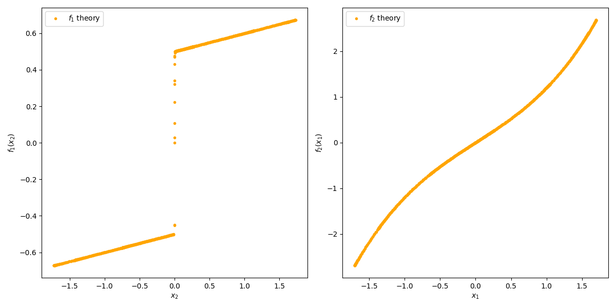
fig, ax = plt.subplots(1, 2, figsize=(12, 6))
ax[0].plot(x1_data, F1(x1_data), '.',color='orange', label="$f_1$ theory")
ax[0].set_xlabel('$x_2$')
ax[0].set_ylabel('$f_1(x_2)$')
ax[0].legend()
ax[1].plot(x2_data, F2(x2_data), '.',color='orange', label="$f_2$ theory")
ax[1].set_xlabel('$x_1$')
ax[1].set_ylabel('$f_2(x_1)$')
ax[1].legend()
plt.tight_layout()
plt.show()


#  Generate database that will be used for training
# Here, we need to define all the variables that appear in eqs variable
df = pd.DataFrame({
    #'t': time_data, # this can be added if eqs include t as an explicit variable but in this example, we encapsulated all the time dependence within F_ext_val
    'x1':x1_data,
    'x2':x2_data,
    'x1_dot':x1_dot_data,
    'x2_dot':x2_dot_data,
    'F_ext': F_ext_val
})

# Define the proposed equation, in this approach, we will use the parametric
# approach where we want to find the ai parameters
eqs = [
    'x1_dot = x2',
    'x2_dot = F_ext - a1 * x2 - a2* tanh(a3*x2)- a4 * x1 - a5 * x1^3',
]

# Using Polynomial method (Poly-CC)
# This method uses Polynomial expansions for the CCs
# First we set the parameters
params_poly={
  'learning_rate': 1e-3,
  'initial_param_guess':[
      {'a3':100},
  ],
  'N_order': 40,
  'n_iter': 4000,
  'eq_weights': [1.0 , 1.0],
  ## post-fine-tuning parameters are in the following:
  'fitting_forw_sim':True,  # Enables the option of refitting the coefficients using forward integr
  'n_iter_outer': 100,      # Max number of function evaluations for the outer loop
  'outer_tol': 1e-6,        # Tolerance for termination in the outer loop
  'params_simul': [
    {'local_funcs': {'F_ext': lambda t: F_ext(t)}},
    {'t_span':t_span},
    {'y0': y0},
    {'t_eval': t_eval},
    {'method': 'LSODA'},
  ],
}
# And here, we train the model
models, evals , scalar_coefs = pycc.train(df=df,equations=eqs,method='Poly',params=params_poly)
# plot obtained functions (characteristic curves CCs)
#x_f1_cc, f1_cc, x_f2_cc, f2_cc = evals
print(scalar_coefs)

x_f1_cc = np.linspace(np.min(x1_data), np.max(x1_data), 200)
x_f2_cc = np.linspace(np.min(x2_data), np.max(x2_data), 200)

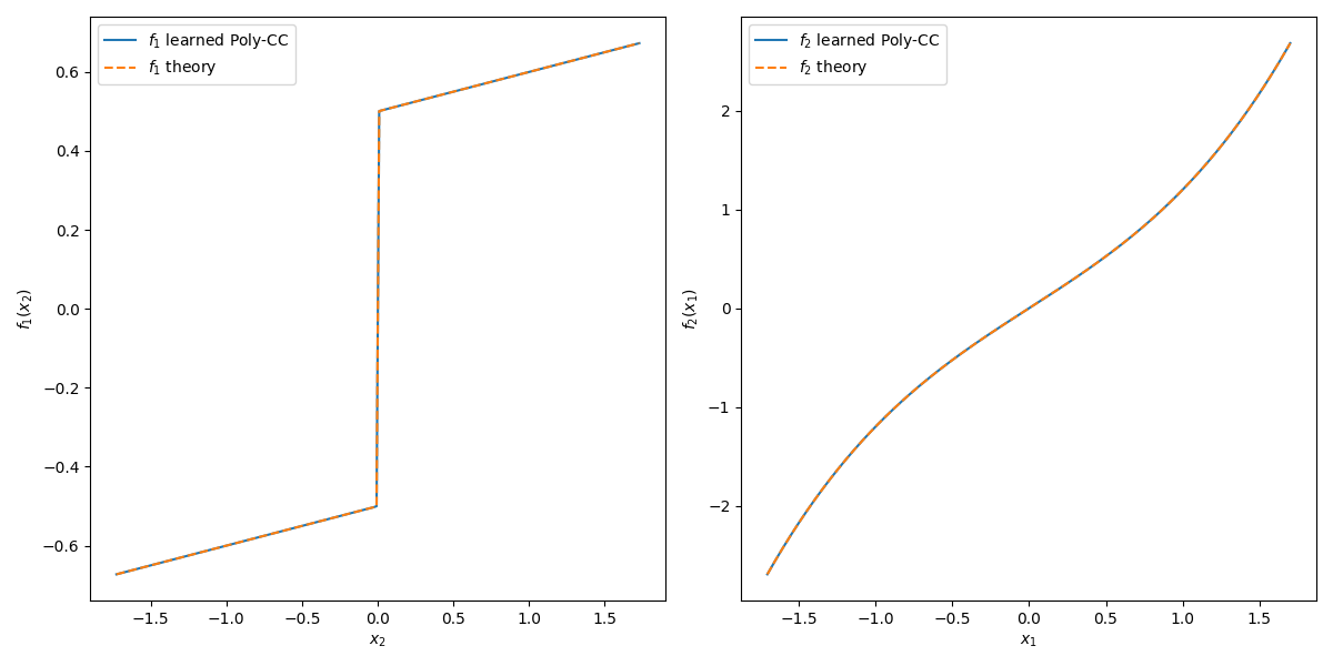
fig, ax = plt.subplots(1, 2, figsize=(12, 6))
ax[0].plot(x_f1_cc, scalar_coefs['a1']*x_f1_cc+scalar_coefs['a2']*np.tanh(scalar_coefs['a3']*x_f1_cc), label='$f_1$ learned Poly-CC')
ax[0].plot(x_f1_cc, F1(x_f1_cc), '--', label="$f_1$ theory")
ax[0].set_xlabel('$x_2$')
ax[0].set_ylabel('$f_1(x_2)$')
ax[0].legend()
ax[1].plot(x_f2_cc, scalar_coefs['a4']*x_f2_cc+scalar_coefs['a5']*x_f2_cc**3, label='$f_2$ learned Poly-CC')
ax[1].plot(x_f2_cc, F2(x_f2_cc), '--', label="$f_2$ theory")
ax[1].set_xlabel('$x_1$')
ax[1].set_ylabel('$f_2(x_1)$')
ax[1].legend()
plt.tight_layout()
plt.show()

params_poly_simul = {
    'models': models, # how we enter evals instead of models
    #'evals':evals, # fi functions obtained from Poly-CC to do interpolation
    'scaling': True,
    'obtained_coefs': scalar_coefs,
    'scalar_params': scalar_coefs,
    'local_funcs': {'F_ext': lambda t: F_ext(t)},
    't_span':t_span,
    'y0': y0,
    't_eval': t_eval,
    'method': 'LSODA',
}

sol,_ = pycc.simulate(eqs, method='Poly', params=params_poly_simul)
print(sol)
time_sim=sol.t
x1=sol.y[0]
x2=sol.y[1]

# Plot solution
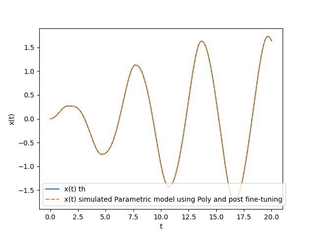
plt.figure()
plt.plot(time_data, x1_data, label="x(t) th")
plt.plot(time_sim, x1,'--', label="x(t) simulated Parametric model using Poly and post fine-tuning")
plt.xlabel('t')
plt.ylabel('x(t)')
plt.legend()
plt.show()