Example 2: 2nd-order ODE
This example presents the application of PyCC to a family of second order systems called as velocity-dependent friction models with external force (which is a generalized Rayleigh-type nonlinear oscillation with velocity-dependent friction and external forcing).
The code follows these steps: 1) it uses the PyCC library to generate the data, 2) it defines a skeleton and uses NN method to train a model, 3) it simulates the model and compares it to the data, 4) it uses the post-processing tool to generate symbolic expressions for the 1D functions obtained with the NN method, 5) it simulates the analytical model by using interpolations of the discovered symbolic expressions.
import pycc
import numpy as np
import pandas as pd
import matplotlib.pyplot as plt

##############################################
# 1) simulate a stick-slip second order system using pycc.simulate()
# 1a) define parameters and functions
alpha=1.0;beta=0.2;delta=0.1;Omega=1.0;
x0=0.0;v0=0.0; y0=[x0,v0] # initial conditions
t_span=(0, 20); t_eval=np.linspace(*t_span, 1000)
def F1_th(x_dot):
    return delta * x_dot + 0.5 * np.tanh(500*x_dot)
def F2_th(x):
    return alpha * x + beta * x**3
def F_ext(t):
    return np.cos(Omega * t)
# 1b) define equation
eqs_th = ['x1_dot = x2',
          'x2_dot = F_ext - f1(x2) - f2(x1)']
# 1c) define simulation parameters
params_th = {
    't_span': t_span,
    'y0': y0,
    't_eval': t_eval,
    'method': 'LSODA',
    'local_funcs': {'f1': lambda t: F1_th(t),'f2': lambda t: F2_th(t),'F_ext': lambda t: F_ext(t)}
}
# 1d) integrate forward the theoretical equation
sol,derivatives = pycc.simulate(eqs_th,method="Theoretical", params=params_th)
# 1e) extract data from theoretical solution
time_data    = sol.t
x1_data      = sol.y[0]
x2_data      = sol.y[1]
x1_dot_data  = derivatives[0]
x2_dot_data  = derivatives[1]
F_ext_val    = F_ext(time_data)
# define database for training
df = pd.DataFrame({
    'x1':x1_data,
    'x2':x2_data,
    'x1_dot':x1_dot_data,
    'x2_dot':x2_dot_data,
    'F_ext': F_ext_val
})


##############################################
# 2) how to train the NN-CC method to identify the model [pycc.train()]
# 2a) propose equations to use for identification (fi functions and ai parameters).
eqs = [
     'x1_dot = x2',
     'x2_dot = F_ext - f1(x2) - f2(x1)'
]
# 2b) define constraints (optional)
constraints = [ # adding prior known information
    {'constraint': 'f2(0)=0'},
    {'constraint': 'f1 odd'},
    {'constraint': 'f2 odd'},
]
# 2c) define training parameters (optional)
params_NN = {
    'neurons': 100,
    'layers':3,
    'lr': 1e-4,
    'epochs': 2000,
    'error_threshold': 1e-6,
    'extrapolation': None,
    'device':'cpu',
    'weight_loss_param': 1e-3,
    'constraints': constraints,
}
# 2d) train/fit/identify the model
models, evals, obtained_coefs = pycc.train(df, eqs,method='NN', params=params_NN)
# plotting obtained functions f1 and f2
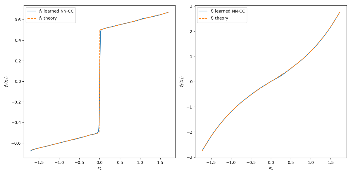
x_f1_cc, f1_cc, x_f2_cc, f2_cc = evals
fig, ax = plt.subplots(1, 2, figsize=(12, 6))
ax[0].plot(x_f1_cc, f1_cc, label='$f_1$ learned NN-CC')
ax[0].plot(x_f1_cc, F1_th(x_f1_cc), '--', label="$f_1$ theory")
ax[0].set_xlabel('$x_2$')
ax[0].set_ylabel('$f_1(x_2)$')
ax[0].legend()
ax[1].plot(x_f2_cc, f2_cc, label='$f_2$ learned NN-CC')
ax[1].plot(x_f2_cc, F2_th(x_f2_cc), '--', label="$f_2$ theory")
ax[1].set_xlabel('$x_1$')
ax[1].set_ylabel('$f_2(x_1)$')
ax[1].legend()
plt.tight_layout()
plt.show()
# Print learned parameters (if any)
if obtained_coefs:
    print("\nLearned scalar parameters:")
    for name, val in obtained_coefs.items():
        print(f"{name} = {val.item():.4f}")

##############################################
# 3) how to simulate the identified model [pycc.simulate()]
print("simulation with NN simul")
# 3a) define simulation parameters
params_NN_simul = {
    'models': models,
    'obtained_coefs': obtained_coefs,
    'local_funcs': {'F_ext': lambda t: F_ext(t)},
    't_span':t_span,
    'y0': y0,
    't_eval': t_eval,
    'method': 'LSODA',  # solve_ivp
    'atol': 1e-8,
    'rtol': 1e-6,
    'check_nan': True
}
# 3b) integrate identified equations
sol,_ = pycc.simulate(eqs, method='NN', params=params_NN_simul)
print("Integration success:", sol.success)
time_sim=sol.t
x1_sim=sol.y[0]
x2_sim=sol.y[1]
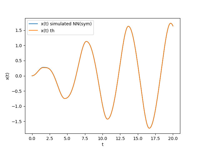
# Identified vs theoretical solution
plt.figure()
plt.plot(time_sim, x1_sim, label="x(t) simulated NN(sym)")
plt.plot(time_data, x1_data, label="x(t) th")
plt.xlabel('t')
plt.ylabel('x(t)')
plt.legend()
plt.show()


##############################################
# 4) Post-processing the identified models with SymbR [pycc.post_processing()]

### Simulation using the NN models
print("simulation with NN simul")
# 3a) define simulation parameters
# Define settings for the PySR fit
pysr_settings = {
    'niterations': 100,
    'populations': 20,
    'binary_operators': ['+', '*', '-'],
    'unary_operators': ['tanh', 'sin','cos'],
    'maxsize': 20
}
# Define the 'params' dictionary for the post-processing function
post_process_params = {
    'evals': evals,
    'pysr': pysr_settings,
    'plot': True,  # This will show the plots of the fits
    'n_eval': 200,   # Generate 200 points for the new evals_sr
}
# Run the post-processing
# This will print the fits and show plots
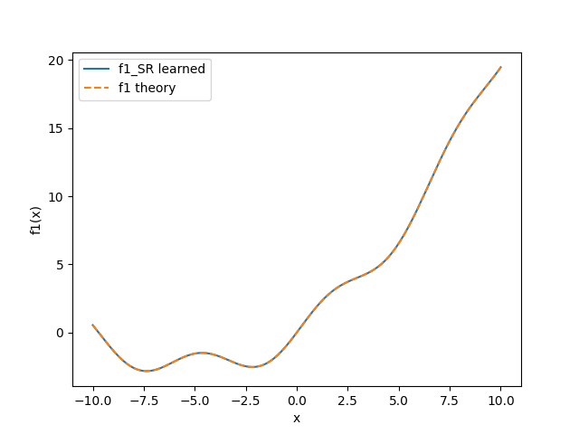
models_sr,evals_sr = pycc.post_processing(eqs, method='SymbR', params=post_process_params)

##############################################
# 5) Simulate the post-processed model using interpolation
params_sim_interp = {
    'evals': evals_sr,          # Use the NN's characteristic curves
    'obtained_coefs': obtained_coefs,  # Use the scalars from the NN fit
    'local_funcs': {'F_ext': F_ext},
    'interp_method': 'pchip',   # Use shape-preserving cubic
    't_span': t_span,
    'y0': y0,
    't_eval': t_eval,
}
# This will simulate the system by interpolating the 'evals_nn' data.
sol, derivs = pycc.simulate(eqs, method='Interp', params=params_sim_interp)
print("Integration success:", sol.success)
time_sim=sol.t
x1_sim=sol.y[0]
x2_sim=sol.y[1]
# Identified vs theoretical solution
plt.figure()
plt.plot(time_sim, x1_sim, label="x(t) simulated NN(sym+postSR)")
plt.plot(time_data, x1_data, label="x(t) th")
plt.xlabel('t')
plt.ylabel('x(t)')
plt.legend()
plt.show()