Example 3: 3rd-order ODE
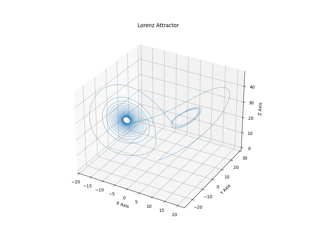
This example uses the PyCC library to simulate a Lorenz system (a set of three coupled, nonlinear ODEs). It then uses three different methods (neural networks, polynomials, and symbolic regression) to discover the equations.
import pycc
import numpy as np
import pandas as pd


#### integration of the theoretical EDO using pycc.id ####
# --- Parameters --- Chaotic solutions
sigma  = 10.0  # a1=10
rho   = 28.0  # a2=28
beta  = 8.0/3.0 # a3~2.666666666
x0     = 0.5
y0     = 0.8
z0     = -0.3
initial_state = [x0, y0, z0]
t_span  = (0, 20)
t_eval  = np.linspace(*t_span, 3000)


#eq1 = 'dxdt = a1 * (y - x)'
#eq2 = 'dydt = x * (a2 - z) - y'
#eq3 = 'dzdt = x * y - a3 * z'
eq1 = 'x1_dot = a1 * (x2 - x1)'
eq2 = 'x2_dot = x1 * (a2 - x3) - x2'
eq3 = 'x3_dot = x1 * x2 - a3 * x3'
eqs_th = [eq1, eq2, eq3]

params_th = {
    't_span': t_span,
    'y0': initial_state,
    't_eval': t_eval,
    'method': 'LSODA',
    'scalar_params': {'a1': sigma,'a2': rho,'a3': beta},
}
# 1d) integrate forward the theoretical equation
sol,derivatives = pycc.simulate(eqs_th,method="Theoretical", params=params_th)
# 1e) extract data from theoretical solution
time_data    = sol.t
x_data      = sol.y[0]
y_data      = sol.y[1]
z_data      = sol.y[2]
dxdt_data  = derivatives[0]
dydt_data  = derivatives[1]
dzdt_data  = derivatives[2]
# --- Plot the results ---
fig = plt.figure(figsize=(10, 8))
ax = fig.add_subplot(111, projection='3d')
ax.plot(x_data, y_data, z_data, lw=0.5)
ax.set_xlabel('X Axis')
ax.set_ylabel('Y Axis')
ax.set_zlabel('Z Axis')
ax.set_title('Lorenz Attractor')
plt.show()
#, method='BDF', rtol=1e-6, atol=1e-8, dense_output=True)
print(sol.status)   # 0 = success, 1 = reached event, -1 = failed
print(sol.message)
# define database for training
df = pd.DataFrame({
    #'t': time_data,
    'x1': x_data,
    'x2': y_data,
    'x3': z_data,
    'x1_dot': dxdt_data,
    'x2_dot': dydt_data,
    'x3_dot': dzdt_data,
})
print(df.head())


####################################
##### define equation to discover/fit
###########################

# --- Define functions as strings ---
def_eq1 = 'x1_dot = a1 * (x2 - x1)'
def_eq2 = 'x2_dot = x1 * (a2 - x3) - x2'
def_eq3 = 'x3_dot = x1 * x2 - a3 * x3'
equations = [def_eq1, def_eq2, def_eq3]

#equation1='x_ddot + f1(x_dot) + f2(x)- F_ext  = 0'
#equation2='f2(x)=0'


########################################
          #### method NN  ####
########################################
#equation='x_ddot + f1(x_dot) + a1*x + a2*x**3 - F_ext = 0'
#equation='x_ddot + a1*x_dot + a2*x + a3*x**3 - F_ext = 0'
constraints = [
    {'constraint': 'f1(0)=0', 'penalty': 1e-2},
   #{'constraint': 'f2(0)=0', 'penalty': 1e-2},
    {'constraint': 'f1 odd', 'penalty': 1e-1, 'eval': 'array','Nval_array':100}, # penaly is optional
    {'constraint': 'f2 odd', 'penalty': 1e-1, 'eval': 'array','Nval_array':100}, # eval=data/array array is default
]
#constraints = [
#    {'constraint': 'f1(0)=0'},
#    {'constraint': 'f2(0)=0'},
#]
parameters_NN = {
    'neurons': 100,
    'lr': 1e-2,
    'epochs': 10000,
    'error_threshold': 1e-6,
    'extrapolation': None,
    'device':'cpu',
    'weight_loss_param': 1e-2,
    # 'param_penalty_weight': 0.0,
    #'constraints': constraints,
    #'eq_weights': [1.0, 1.0]
}


models, evals, obtained_coefs = pycc.train(df, equations,method='NN', params=parameters_NN)


# The key is to loop through the evals list in steps of 2
num_functions = len(evals) // 2
if num_functions == 1:
    x_f1_cc, f1_cc = evals
    plt.figure()
    plt.plot(x_f1_cc, f1_cc, label='f1 learned')
    #plt.plot(x_data,np.ones(x_data)*sigma, '--', label="f1 theory")
    plt.xlabel('x')
    plt.ylabel('f1(x)')
    plt.legend()
    plt.figure()
    plt.show()
elif num_functions == 2:
    x_f1_cc, f1_cc, x_f2_cc, f2_cc = evals
elif num_functions == 3:
    x_f1_cc, f1_cc, x_f2_cc, f2_cc, x_f3_cc, f3_cc = evals

# Print learned parameters (if any)
if obtained_coefs:
    print("\nLearned scalar parameters:")
    for name, val in obtained_coefs.items():
        print(f"{name} = {val.item():.4f}")


#models, evals = pycc.train(df, equation, neurons=50, lr=1e-2, epochs=2000)

## Plot learned functions
#x_f1_cc, f1_cc, x_f2_cc, f2_cc = evals
#plt.figure()
#plt.plot(x_f1_cc, f1_cc, label='f1 learned')
#plt.plot(x_dot_data,F1_th, '--', label="f1 theory")
#plt.xlabel('x_dot')
#plt.ylabel('f1(x_dot)')
#plt.legend()
#plt.figure()
#plt.plot(x_f2_cc, f2_cc, label='f2 learned')
#plt.plot(x_data, F2_th, '--', label="f2 theory")
#plt.xlabel('x')
#plt.ylabel('f2(x)')
#plt.legend()
#plt.show()


## integrate identified equations with NN-CC


########################################
          #### method Poly  ####
########################################
print("computing Poly")
params_poly={
  'scaling': False,
  'constraints': [
      #  {'constraint': 'f1(0)=0'},#,'penalty':1e1},
        #{'constraint': 'f2(0)=0'},
        #{'constraint': 'f1 odd'},
        #{'constraint': 'f2 odd'}
    ],
  #'eq_weights':[1.0,1.0]
}
models, evals , scalar_coefs = pycc.train(
    df=df,
    equations=equations,
    method='Poly', #method='Poly_linear',
    params=params_poly
)
if len(evals) == 2:
    x_f1_cc, f1_cc = evals
elif len(evals) == 4:
    x_f1_cc, f1_cc, x_f2_cc, f2_cc = evals

# The key is to loop through the evals list in steps of 2
num_functions = len(evals) // 2
if num_functions == 1:
    x_f1_cc, f1_cc = evals
elif num_functions == 2:
    x_f1_cc, f1_cc, x_f2_cc, f2_cc = evals
elif num_functions == 3:
    x_f1_cc, f1_cc, x_f2_cc, f2_cc, x_f3_cc, f3_cc = evals


########################################
          #### method SymbR  ####
########################################
#def_eq1 = 'dxdt = a1 * (y - x)'
def_eq1 = 'x1_dot = f1(x1) * (x2 - x1)'
def_eq2 = 'x2_dot = x1 * (a2 - x3) - x2'
def_eq3 = 'x3_dot = x1 * x2 - a3 * x3'
equations = [def_eq1, def_eq2, def_eq3]

params_SymbR = {
  'pysr': {
    'niterations': 100,
    'unary_operators': ['tanh'],
    'binary_operators': ['+','-','*'],
    'maxsize': 12,
    'populations':10,
    'model_selection': 'best', # 'best' , 'accuracy' , 'score'
    'verbosity': 0
  },
  'N_fit_points': 200,
  'max_iterations': 15,
}


models, evals , scalar_coefs = pycc.train(
    df=df,
    equations=equations,
    method='SymbR',
    params=params_SymbR
)


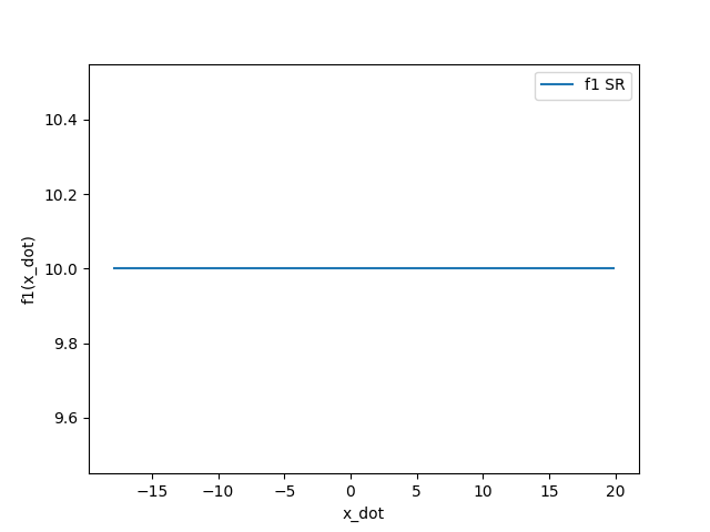
if len(evals) == 2:
    x_f1_cc, f1_cc = evals
    # then your plotting code:
    plt.figure()
    plt.plot(x_f1_cc, f1_cc, label='f1 SR')
    plt.xlabel('x_dot')
    plt.ylabel('f1(x_dot)')
    plt.legend()
    plt.show()
elif len(evals) == 4:
    x_f1_cc, f1_cc, x_f2_cc, f2_cc = evals
    # then your plotting code:
    x_f1_cc, f1_cc, x_f2_cc, f2_cc = evals
    plt.figure()
    plt.plot(x_f1_cc, f1_cc, label='f1 SR')
    plt.plot(x_dot_data,F1_th, '--', label="f1 theory")
    plt.xlabel('x_dot')
    plt.ylabel('f1(x_dot)')
    plt.legend()
    plt.figure()
    plt.plot(x_f2_cc, f2_cc, label='f2 SR')
    plt.plot(x_data, F2_th, '--', label="f2 theory")
    plt.xlabel('x')
    plt.ylabel('f2(x)')
    plt.legend()
    plt.show()