Example 4: 1st-order ODE with f in denominator

This example presents the application of pyCC to a family of first-order systems as discussed in Ref.[Gonzalez2023]. In this case, for training the system is useful to rewrite the system with the unknown functions in the numerator.

import pycc
import numpy as np
import pandas as pd
import matplotlib.pyplot as plt
import matplotlib.ticker as ticker
from scipy.integrate import solve_ivp
from scipy.signal import savgol_filter

# --- Parameters ---
beta   = 0.2
delta  = 0.1
F0     = 3.0
Omega  = 1.0
x0     = 0.5
t_span  = (0, 50)
t_eval  = np.linspace(*t_span, 1000)
y0      = [x0]  # initial conditions

#theoretical functions
def F1(x):
    return delta * x + beta* np.sin(3*x)
def F2(x):
    return 1+np.abs(x) # np.sin(x)
def F_ext(t):
    return F0 * np.cos(Omega * t)

print(f"beta={beta}, delta={delta}")
print(f"Omega={Omega}, F0={F0}, $x_0$={x0}")


########################
##### integration using pycc of theoretical equation
#########################
# equation involved:
## Fext = f1(x) +f2(x) x'

# Parameters for simulation
params_th = {
    "t_span": t_span,
    "y0": y0,  # x, x_dot, x_ddot
    "t_eval": t_eval,
    "method": "LSODA",
    "local_funcs": {"f1": lambda t: F1(t), "f2": lambda t: F2(t), "F_ext": lambda t: F_ext(t)}
}

#equation=['f1(x) + x_dot*f2(x) = F_ext']
equation=['x_dot = (F_ext - f1(x))/f2(x)']

#equation = "x_ddot + f1(x) + f2(x) - F_ext = 0"
sol,der = pycc.simulate(equation,method="Theoretical", params=params_th)


# 1e) extract data from theoretical solution
time_data  = sol.t
x1_data     = sol.y[0]
x1_dot_data=der[0]
F_ext_val  = F_ext(time_data)


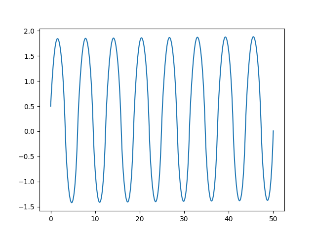
plt.plot(time_data,x1_data)
plt.show()

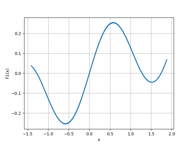
F1_th=F1(x1_data)
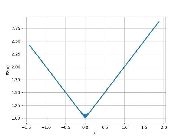
F2_th=F2(x1_data)

plt.plot(x1_data, F1_th)
plt.xlabel("x")
plt.ylabel("F1(x)")
plt.grid(True)
plt.show()

plt.plot(x1_data, F2_th)
plt.xlabel("x")
plt.ylabel("F2(x)")
plt.grid(True)
plt.show()


# define database for training
df = pd.DataFrame({
    'x':x1_data,
    'x_dot':x1_dot_data,
    'F_ext': F_ext_val
})

# define the equation for training with functions in the numerators
eq_train=['f1(x) + x_dot*f2(x) = F_ext']

########################################
          #### method NN  ####
########################################
constraints = [
    {'constraint': 'f1(0)=0'},
    {'constraint': 'f1 odd'},
    {'constraint': 'f2 odd'},
]
parameters_NN = {
    'neurons': 100,
    'lr': 1e-4,
    'epochs': 2000,
    'error_threshold': 1e-6,
    'extrapolation': None,
    'weight_loss_param': 1e1,
    #'constraints':constraints,
}

models, evals, obtained_coefs = pycc.train(
    df=df,
    equations=eq_train,
    method='NN',
    params=parameters_NN
)


x_f1_cc, f1_cc, x_f2_cc, f2_cc = evals

plt.figure()
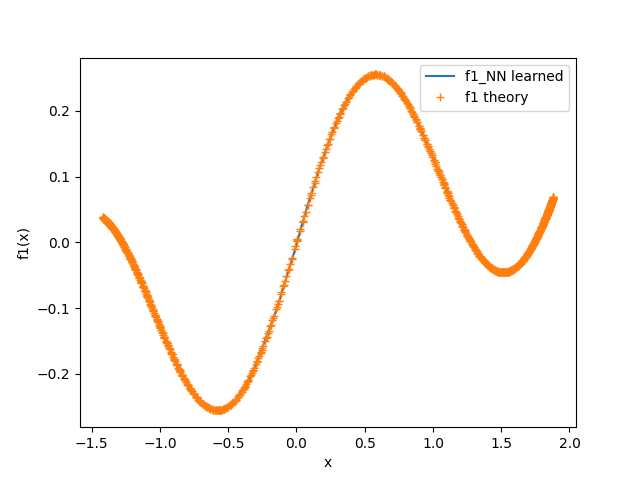
plt.plot(x_f1_cc, f1_cc, label='f1_NN learned')
plt.plot(x1_data,F1_th, '+', label="f1 theory")
plt.xlabel('x')
plt.ylabel('f1(x)')
plt.legend()
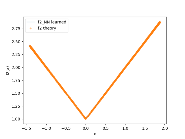
plt.figure()
plt.plot(x_f2_cc, f2_cc, label='f2_NN learned')
plt.plot(x1_data, F2_th, '+', label="f2 theory")
plt.xlabel('x')
plt.ylabel('f2(x)')
plt.legend()
plt.show()

# Print learned parameters (if any)
if obtained_coefs:
    print("\nLearned scalar parameters:")
    for name, val in obtained_coefs.items():
        print(f"{name} = {val.item():.4f}")



############### now simulate with NN-CC #########
# WARNING: for simulation we must redefine the train equations
# as a set of equivalent first order equations like the following:
#eq_train=['f1(x) + x_dot*f2(x) = F_ext']
eq_simulate=['x_dot = (F_ext - f1(x))/f2(x)']

print("simulation with NN simul")
params_NN_simul = {
    'models': models,
    'obtained_coefs': obtained_coefs,
    'local_funcs': {'F_ext': lambda t: F_ext(t)},
    't_span':t_span,
    'y0': y0,
    't_eval': t_eval,
    'method': 'LSODA',  # solve_ivp
    'atol': 1e-8,
    'rtol': 1e-6,
    'check_nan': True
}
sol,_ = pycc.simulate(eq_simulate, method='NN', params=params_NN_simul)
print("Integration success:", sol.success)
time_sim=sol.t
x1_sim=sol.y[0]

# Identified vs theoretical solution
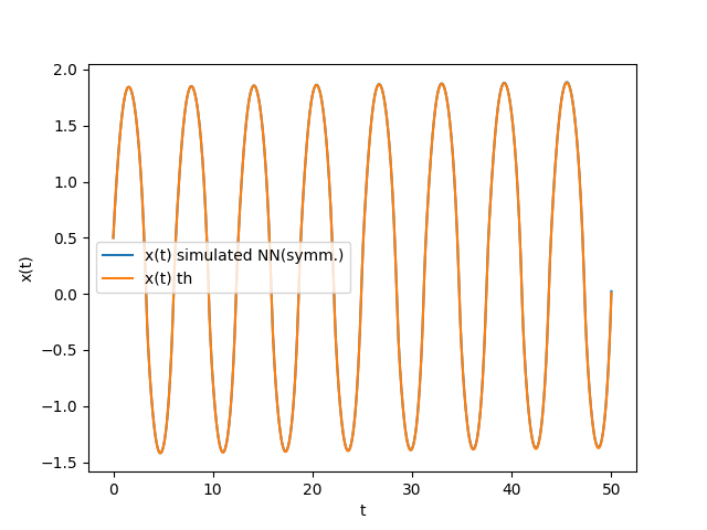
plt.figure()
plt.plot(time_sim, x1_sim, label="x(t) simulated NN(symm.)")
plt.plot(time_data, x1_data, label="x(t) th")
plt.xlabel('t')
plt.ylabel('x(t)')
plt.legend()
plt.show()


## now we will test
########################################
          #### method Poly  ####
########################################
print("computing Poly")
params_poly={
  'scaling': True,
  'n_iter':2000,
}
models, evals , scalar_coefs = pycc.train(
    df=df,
    equations=eq_train,
    method='Poly',
    params=params_poly
)

x_f1_cc, f1_cc, x_f2_cc, f2_cc = evals
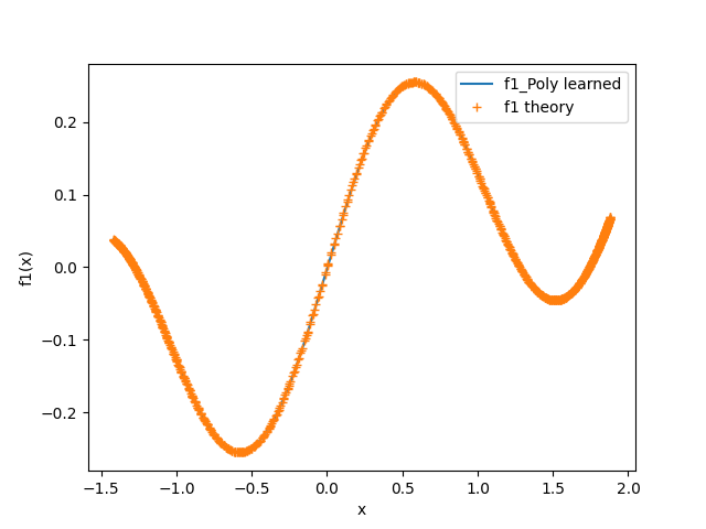
plt.figure()
plt.plot(x_f1_cc, f1_cc, label='f1_Poly learned')
plt.plot(x1_data,F1_th, '+', label="f1 theory")
plt.xlabel('x')
plt.ylabel('f1(x)')
plt.legend()
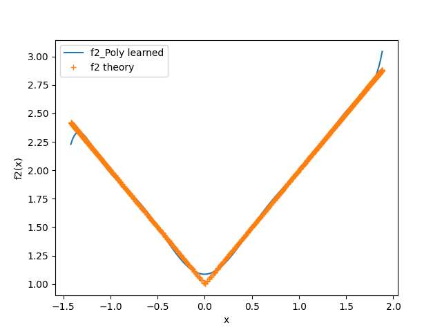
plt.figure()
plt.plot(x_f2_cc, f2_cc, label='f2_Poly learned')
plt.plot(x1_data, F2_th, '+', label="f2 theory")
plt.xlabel('x')
plt.ylabel('f2(x)')
plt.legend()
plt.show()



########################################
          #### method SymbR  ####
########################################
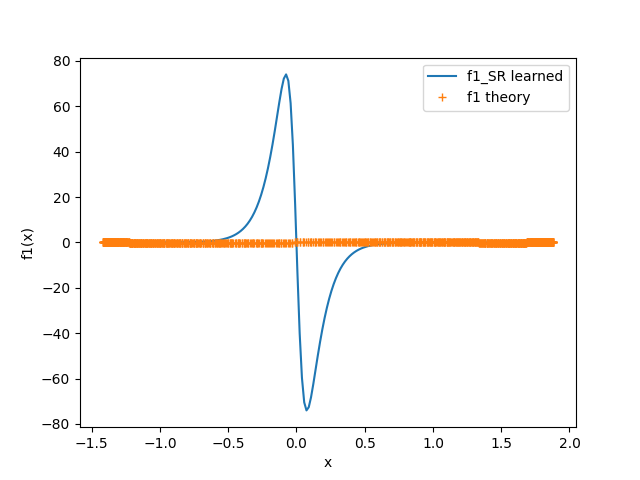
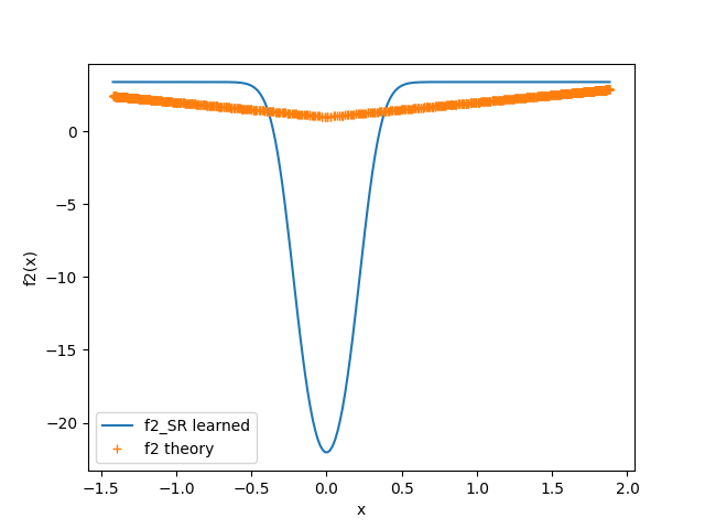
# symbolic regression method is not as useful
# as NN in this example

params_SymbR = {
  'pysr': {
    'niterations': 100,
    'unary_operators': ['tanh'],
    'binary_operators': ['+','-','*'],
    'maxsize': 12,
    'populations':10,
    'model_selection': 'best', # 'best' , 'accuracy' , 'score'
    'verbosity': 0
  },
  'N_fit_points': 200,
  'max_iterations': 15,
}

models, evals , scalar_coefs = pycc.train(
    df=df,
    equations=eq_train,
    method='SymbR',
    params=params_SymbR
)

x_f1_cc, f1_cc, x_f2_cc, f2_cc = evals

plt.figure()
plt.plot(x_f1_cc, f1_cc, label='f1_SR learned')
plt.plot(x1_data,F1_th, '+', label="f1 theory")
plt.xlabel('x')
plt.ylabel('f1(x)')
plt.legend()
plt.figure()
plt.plot(x_f2_cc, f2_cc, label='f2_SR learned')
plt.plot(x1_data, F2_th, '+', label="f2 theory")
plt.xlabel('x')
plt.ylabel('f2(x)')
plt.legend()
plt.show()